From Source Code to Executable

Originally published in Japanese at https://zenn.dev/ymotongpoo/books/go-ebpf-primer/viewer/15-source_to_binary.

Chapter 2 described instructions stored at addresses in memory. The executable file supplies that sequence. This chapter follows source code through compilation and linking, then examines the finished file.

The tools go tool objdump and go tool nm expose the machine code and the table that maps names to addresses. The hurdle chapters use both, along with the executable’s internal structure.

From source to machine code

When you build Go source code, you get a binary containing a sequence of machine-code instructions. Machine code is the byte-level representation of the “smallest units of work a CPU can do” that we saw in Chapter 2. The instructions are laid out in order from the start, and each one has an address. Execution is the repeated cycle of fetching the instruction at the address the PC points to, executing it, and advancing the PC.

Somewhere in this transformation, the function you wrote in main.go becomes “a sequence of instructions plus the address where they live”. Function names and variable names are, as a rule, not carried over into the world of machine code.

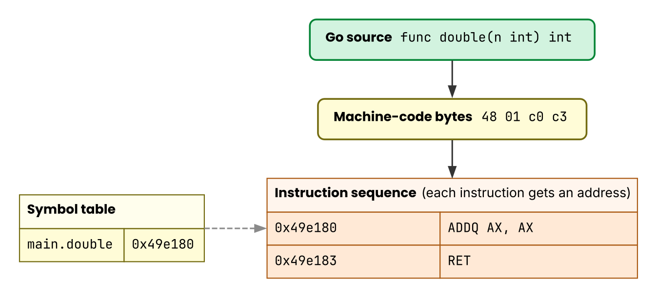Figure 1: Solid arrows show the direction of transformation. The dashed arrow shows the symbol table looking up an address from a name; it is a reference rather than a transformation.

Disassembly

Turning a sequence of machine-code bytes back into human-readable instruction notation is called disassembly. Go ships with go tool objdump.

This book does not require you to write assembly. In disassembly output, the lines marked with arrows or annotations contain the parts used in the explanation.

The following small function provides an example. //go:noinline tells the compiler not to expand the function, leaving it as a call; Chapter 5 explains why.

• Open in the Go Playground

package main

import "fmt"

//go:noinline
func double(n int) int {
	return n * 2
}

func main() {
	fmt.Println(double(21))
}

Build it and disassemble main.double. The output below is from a binary built with GOOS=linux GOARCH=amd64. Even if your machine runs macOS or Windows, building with these two environment variables lets you observe the same thing.

$ GOOS=linux GOARCH=amd64 go build -o demo main.go
$ go tool objdump -s 'main\.double$' demo
TEXT main.double(SB) .../main.go
  main.go:7   0x49e180   4801c0   ADDQ AX, AX   ← computes n*2
  main.go:7   0x49e183   c3       RET           ← returns from the function

The columns, from left to right, are the source line number, instruction address, machine-code bytes, and human-readable instruction notation. The Go expression n * 2 became ADDQ AX, AX, which adds AX to itself. RET returns from the function.

Look at the bytes column. 4801c0 is three bytes and c3 is one byte: the instructions are not all the same length. What’s more, the byte sequence itself contains no markers saying “this instruction runs from here to here”. A disassembler has no choice but to interpret one instruction at a time, starting from the beginning. This property shows up again in Hurdle 1, as actual OBI code.

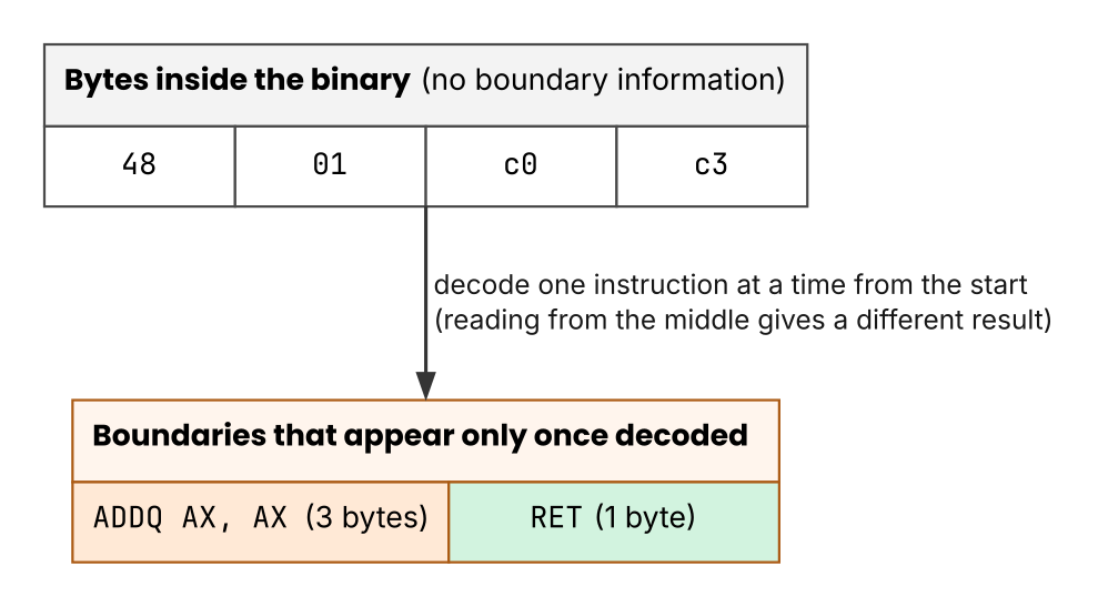Figure 2: The arrow shows the direction interpretation proceeds. The same four bytes only separate into “a three-byte instruction and a one-byte instruction” once you interpret them in order from the start. Start reading from a byte in the middle and you get a different interpretation.

The symbol table

Machine code does not carry names. A separate symbol table maps them to addresses, including the earlier fact that main.double starts at 0x49e180. You can inspect it with go tool nm.

$ go tool nm demo | grep 'main\.double'
  49e180 T main.double

This table is why go tool objdump can accept a function name and disassemble only that function. For an external tool that needs to hook a function’s entry, it is also the first place to look up the function’s address from its name.

Static linking and dynamic linking

Compilation happens per source component (in Go, per package). The step that combines the machine code produced for each component into a single executable, deciding the final address where each function will live, is linking, and the program that does it is the linker.

There are two ways to combine libraries. Static linking copies the machine code of every library you use wholesale into the executable. Dynamic linking leaves each library as a separate file called a shared library and binds them at run time. The typical C program takes the latter approach: the machine code of, say, the standard C library (libc) functions lives outside the executable, and their addresses are decided at run time.

Go’s linker chooses static linking by default. Chapter 6 explains how this affects instrumentation.

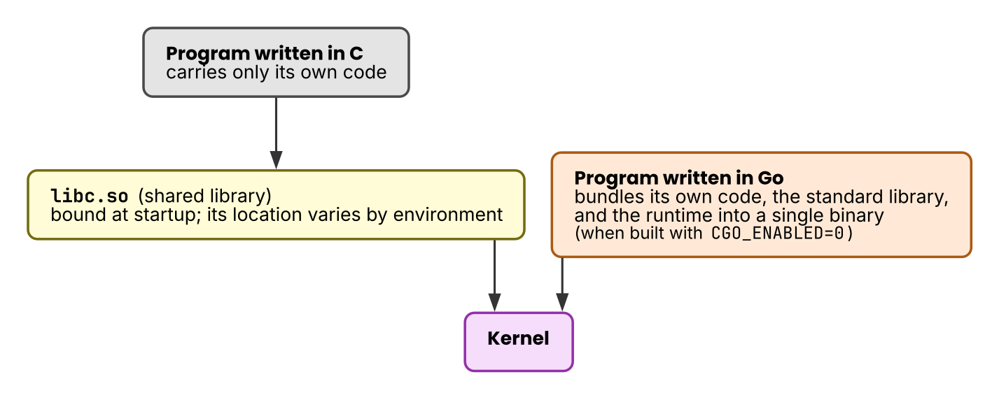Figure 3: Arrows show the direction of dependency. A C process resolves its shared-library dependencies at run time; a Go binary has no such step.

ELF sections

Executable files on Linux use a format called ELF. Inside, the file is divided into sections: machine code goes in .text, constants in .rodata, and the symbol table we just saw in .symtab.

A Go binary contains two more Go-specific things: .gopclntab, a table for looking up function names and line numbers from addresses, and a build-info blob recording the Go version and the list of dependency modules. The Go runtime itself reads .gopclntab to assemble stack traces on panic.

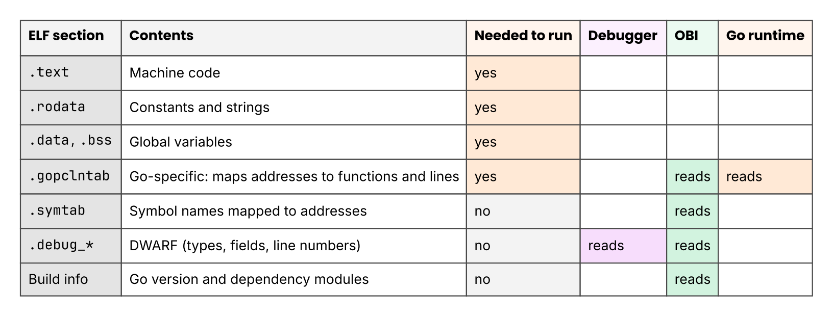Figure 4: A table of who needs which section. Only .text is needed for execution itself; the rest is information for whoever reads the file.

How an executable gets loaded into memory

The “text segment” from Chapter 3 is the in-memory mapping of the executable’s .text section. The bytes originate in the file on disk and appear in the running process through this mapping.

The kernel does not copy the whole file into physical memory at startup. Instead, it records in the mapping table that a range of virtual addresses corresponds to bytes in the executable. The table works in fixed-size units called pages (normally 4KB on Linux). A page reaches physical memory when the CPU first tries to execute an instruction on it¹, so startup does not wait for the entire executable to load.

Another consequence of this scheme is sharing. In the Chapter 3 experiment, two processes started from the same executable (PIDs 25 and 31) had independent virtual address spaces. Even so, their .text pages can share one copy in physical memory. Independent virtual addresses can map to the same physical page. No matter how many instances of a program you start, physical memory needs only one copy of its .text pages².

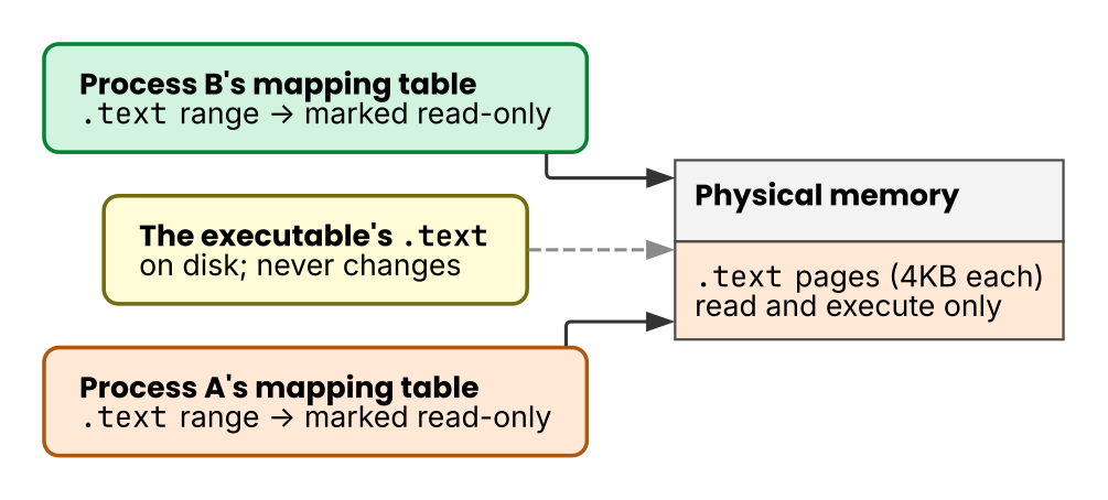Figure 5: Solid arrows show where the mapping tables point; the dashed arrow shows reading from the file. The two processes’ virtual addresses are independent, but their .text mappings may point at the same physical page.

Sharing works because .text pages are read-only. The mapping table records both the physical page and its permissions: “reading and executing allowed, writing not”. If one process rewrote a shared page, it would change every process using that page. The permission prevents such writes.

Some tools do need to modify these pages. A debugger, for instance, modifies a running process’s machine code to plant breakpoints. The kernel supports this through copy-on-write. It leaves the shared page alone, makes a private copy of just the one page to be modified, modifies the copy, and repoints that process’s mapping table at the copy. Neither the file on disk nor the original shared page changes.

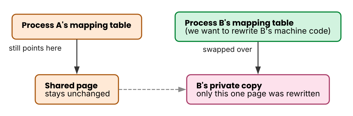Figure 6: Solid arrows show where the mapping tables point; the dashed arrow shows the copy being made. Only the writing process’s mapping table now points at the copy; the original page and the file on disk are unchanged.

Inserting an observation point into a running program from the outside is built on this same mechanism. The concrete details come in Chapter 7.

DWARF

Chapter 2 noted that struct field names vanish from machine code after compilation. Even so, a debugger can display r.count, because the compiler leaves behind debug information called DWARF. It occupies ELF sections whose names start with .debug_³.

Figure 7: Arrows show references. Running memory contains nothing but bytes, but DWARF holds the mapping “this field of this type is this many bytes from the start”, so the debugger can display it by name.

The same information is useful to external instrumentation tools. An instrumentation tool reads .gopclntab or the symbol table to learn where functions are, DWARF to learn where fields are, and the build info to identify the relevant versions.

The program runs without DWARF or the symbol table. Building with -ldflags="-s -w" drops .symtab and DWARF, reducing the file size. Chapter 13 measures the effect on instrumentation.

Key points for the hurdles

• Machine-code bytes carry no instruction boundaries; the only way to interpret them is in order from the start.
• A function’s address can be found from its name via the symbol table or .gopclntab.
• The mapping from field names to offsets survives only in DWARF, and -s -w erases it.
• Machine-code pages are read-only and shared between processes; modifying one means swapping in a process-private copy (copy-on-write).

Exercises

1. Build any Go program, disassemble main.main with go tool objdump -s 'main\.main$', and count how many RET instructions there are.
2. In the output of go tool nm, how many of the functions you wrote (symbols starting with main.) appear? If a small function you’re sure you wrote is missing, what do you think happened? (Hint: Chapter 5 covers it.)